Beer, Evaluation of Final Product and Filtration Efficiency
The use of the Multisizer 3 provides a fast, easy, accurate and automatic method to determine the particle content in beer. The use of this instrument also provides reliable results not dependent on the operator’s judgment making it possible to compare data from different work shifts and/or breweries.
SIGNIFICANCE
The determination of particle concentration in beers is important for evaluating and/or correcting several steps during the brewing process and finishing of the product.- Evaluation of the Final Product. Each kind of beer has its own characteristics and distinctive flavor; these properties will be influenced to some extent by the content and size distribution of particles present in the final product.The stability and therefore the shelf life of beer are also affected by its particle content.
- Evaluation of Chill Haze Effect. This is the most common, and in some sense, the most important type of beer hazesince it is relevant to many beer types. As the name suggests, this haze appears when the beer is suitably chilled; the haze disappears upon warming. The temperatures at which the haze appears and disappears depend on the physical stability of the beer.The more stable the beer, the closer to 0 °C before chill haze occurs.The haze involves complexes of highmolecularweight proteins and polyphenols (tannins). These compounds form weak, temperature sensitive
hydrogen bonds that are broken as the beer’s temperature increases, allowing the resulting compounds to form a complex with water molecules and go into solution. - Filtration Efficiency. Brewers have been using some type of filtration for centuries. If properly used, it can serve as an effective nonadditive tool in beer clarification. Filtration is used in conjunction with fining agents to render beer brilliantly clear and stable with respect to temperature changes.
In this paper we will refer to the evaluation of the final product and filtration efficiency.
EVALUATION OF FINAL PRODUCT
INSTRUMENT SET UP AND CALIBRATION
A 50 µm aperture tube is used for the evaluation of the final product.The linear dynamic range for any aperture is 2% to 60% of its size, i.e. a 50 µm aperture tube will be capable of analyze the particle concentration and size distribution from 1 µm to 30 µm. Set up and calibrate the instrument according to the Multisizer 3 Operator’s Manual. For determining particle concentration the control mode for the instrument must be Volumetric Mode, select 500 µL.
PROCEDURE
- Running a Background
Entering background information in the Multisizer 3 Software. By entering the background information, the software will be able to calculate the concentration of particles in the Isoton.
- Sample Volume: 20 mL
- Electrolyte Volume: 0
- Analytical Volume 500µL

- Place 20 mL of Isoton® II in an Accuvette® II.
- Place into the analyzer the Accuvette® II containing the Isoton, flush the aperture tube before the run.
- On the Multisizer software set the background. The background will be automatically subtracted from all subsequent
- Analyzing the Sample
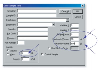
- Entering sample information in the Multisizer 3 Software.
Enter the required sample information in the software: analytical volume electrolyte (Isoton) volume and volume of beer used for the analysis. By entering the sample information, the software will be able to calculate the concentration of particles in the beer.
- Sample Volume: Enter the amount of sample to be use in the analysis
- Electrolyte Volume: Enter the amount of Isoton to be use in the analysis
- Analytical Volume 500 µL
- Sample preparation
After removing gas from the beer, measure exactly 15 mL of Isoton® II into a 20 mL Accuvette® II. Pipette 5.0 mL of beer into the Isoton, these quantities may be different according to the kind of beer, for example for Wheat Ales a smaller amount of sample and more Isoton will be needed. Cap the Accuvette and stir gently to dissolve thoroughly without creating bubbles. Prepare each sample at the moment it will be analyzed. - Place into the analyzer the Accuvette® II containing the sample, flush the aperture tube before the analysis.
- After each run rinse the aperture and electrode before proceeding to the next sample.
- Entering sample information in the Multisizer 3 Software.
- Reporting the results
Results are reported as the total number of particles per mL from 1 to 30 µm and /or particles per mL larger than 1, 2, 3, 4, 5, 10, 15 and 20 µm.
| Particles / mL Larger than | ||||||||
| 1 µm | 2 µm | 3 µm | 4 µm | 5 µm | 10 µm | 15 µm | 20 µm | |
| BECK'S | 10.213 | 2.493 | 1.012 | 538 | 281 | 88 | 51 | 7 |
| BUDWEISER | 16.950 | 1.776 | 697 | 426 | 341 | 183 | 110 | 44 |
| COORS LIGHT | 11.731 | 1.702 | 586 | 273 | 154 | 38 | 16 | 0 |
| CORONA EXTRA | 3.601 | 751 | 377 | 231 | 147 | 59 | 29 | 11 |
| FULLER'S LONDON PRIDE | 744.862 | 107.715 | 35.884 | 16.347 | 8.423 | 693 | 118 | 24 |
| GRANT'S IPA | 330.673 | 58.915 | 15.908 | 5.800 | 2.655 | 205 | 48 | 9 |
| HEINEKEN | 81.292 | 13.888 | 5.302 | 2.968 | 2.071 | 877 | 354 | 76 |
| MILLER LITE | 3.144 | 747 | 378 | 298 | 217 | 76 | 45 | 14 |
| MILLER MDG | 12.638 | 1.845 | 456 | 181 | 110 | 22 | 4 | 0 |
| PRESIDENTE | 29.508 | 5.801 | 2.332 | 1.177 | 615 | 124 | 62 | 23 |
| SAMUEL ADAMS | 352.452 | 80.701 | 27.613 | 12.089 | 6.204 | 700 | 133 | 32 |
| SAM ADAMS WINTER LAGER | 87.196 | 12.763 | 4.501 | 2.048 | 961 | 69 | 7 | 0 |
| SINGHA | 99.980 | 24.166 | 9.879 | 4.857 | 2.678 | 255 | 37 | 12 |
| THE KNIGHT'S ALE (WHITE ALE) | 15.36 x 10⁶ | 1.545 x 10⁶ | 1.368 x 10⁶ | 1.278 x 10⁶ | 661.568 | 1.654 | 306 | 79 |
| Particles/ml 1-30 µm) | Particles/ml 1-30 µm) | ||
| Beck’s (Germany) | 10,213 | Miller Lite (USA) | 3,144 |
| Budweiser (USA) | 16,950 | Miller MGD | 12,638 |
| Coors Light (USA) | 11,731 | Presidente (Dominican Republic) | 29,508 |
| Corona Extra (Mexico) | 3,601 | Samuel Adams (USA) | 352,452 |
| Fuller’s London Pride (UK) | 744,862 | Sam.Adams Winter Lager (USA) | 87,196 |
| Grant’s IPA (USA) | 330,673 | Singha (Thailand) | 99,980 |
| Heineken (Holland) | 81,292 | The Knight’s Ale (Belgium White Ale) | 15.36 x 10⁶ |
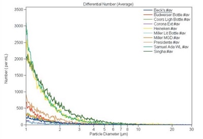
The above data does not represent by any means a comparison for different brands of beer.The samples were randomly selected from brands and kinds of beers available at the market, therefore they have different characteristics and they have been manufactured at different dates and stored under diverse conditions and length of time.The only purpose of this table and following graphs is to show how the results are reported.
DETERMINATION OF SIZE AND CONCENTRATION OF PARTICLES IN BEER FINAL PRODUCT
Comparison Graph for Different Kinds of Beer
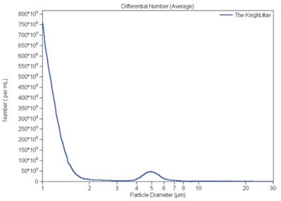
Belgian Wheat Ale
FILTRATION EFFICIENCY
Set up the instrument and follow the same procedure described for the final product steps 1 through 2.4. Perform the analysis for beer getting into the filter and coming out from the filter.
REPORTING THE RESULTS
The efficiency of the filter is determined by comparing the results before and after filtration.The amount of particles removed as a percentage of the particles present before the filtration gives the percentage of efficiency.
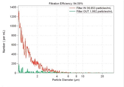
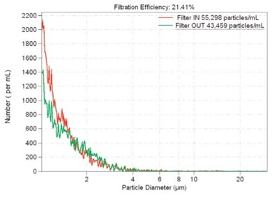
The filtration process may also be monitored for specific size ranges.The total number of particles removed not always provide a complete picture of a filtration deficiency, sometimes it is necessary to target certain size range for adjusting the filtration process.
| Particle Diameter (µm) | Filter IN Number per mL larger than |
Filter OUT Number per mL larger than |
Efficiency (%) |
| 1 | 35.296 | 1.875 | 94.68 |
| 2 | 5.427 | 744 | 86.29 |
| 3 | 1.560 | 327 | 79.02 |
| 4 | 498 | 135 | 72.95 |
| 5 | 244 | 77 | 68.30 |
| 10 | 56 | 19 | 66.66 |
| 15 | 22 | 8 | 63.61 |
| 20 | 4 | 0 | 100 |
Helpful Links
-
Reading Material
-
Application Notes
- 17-Marker, 18-Color Human Blood Phenotyping Made Easy with Flow Cytometry
- 21 CFR Part 11 Data Integrity for On-line WFI Instruments
- 8011+ Reporting Standards Feature and Synopsis
- Air Particle Monitoring ISO 21501-4 Impact
- Automated Cord Blood Cell Viability and Concentration Measurements Using the Vi‑CELL XR
- Biomek Automated NGS Solutions Accelerate Genomic Research
- Biomek i-Series Automation of the Beckman Coulter GenFind V3 Blood and Serum DNA Isolation Kit
- Preparation and purification of carbon nanotubes using an ultracentrifuge and automatic dispensing apparatus, and analysis using an analytical centrifuge system
- Viability Assessment of Cell Cultures Using the CytoFLEX
- Classifying a Small Cleanroom using the MET ONE HHPC 6+
- Clean Cabinet Air Particle Evaluation
- Recommended cleaning procedure for the exterior surface of the MET ONE 3400+
- Counting Efficiency: MET ONE Air Particle Counters and Compliance to ISO-21501
- Critical Particle Size Distribution for Cement using Laser Diffraction
- Detecting and counting bacteria with the CytoFLEX research flow cytometer: II-Characterization of a variety of gram-positive bacteria
- Efficient kit-free nucleic acid isolation uses a combination of precipitation and centrifugation separation methods
- Echo System-Enhanced SMART-Seq v2 for RNA Sequencing
- Grading of nanocellulose using a centrifuge
- Grading of pigment ink and measurement of particle diameter using ultracentrifugation / dynamic light scattering
- How to Use Violet Laser Side Scatter Detect Nanoparticle
- HRLD Recommended Volume Setting
- Particle Size Analysis Simple, Effective and Precise
- Flow Cytometric Analysis of auto-fluorescent cells found in the marine demosponge Clathria prolifera
- MET ONE Sensor Verification
- Metal colloid purification and concentration using ultracentrifugation
- Separation and purification of metal nanorods using density gradient centrifugation
- Miniaturized and High-Throughput Metabolic Stability Assay Enabled by the Echo Liquid Handler
- Minimal Sample to Sample Carry Over with the HIAC 8011+
- Modern Trends in Non‐Viable Particle Monitoring during Aseptic Processing
- Particle diameter measurement of a nanoparticle composite - Using density gradient ultracentrifugation and dynamic light scattering
- Identification of Circulating Myeloid Cell Populations in NLRP3 Null Mice
- Optimizing the HIAC 8011+ Particle Counter for Analyzing Viscous Fluids
- Particle testing in cleanroom high-pressure gas lines to ISO 14644 made easy with the MET ONE 3400 gas calibrations
- Pharma Manufacturing Environmental Monitoring
- Pharma Manufacturing Paperless Monitoring
- Analysis of plant genome sizes using flow cytometry: a case study demonstrating dynamic range and measurement linearity
- Calibrating the QbD1200 TOC Analyzer
- Detection Limit
- Vibrio Natriegens Process Scale-up
- A fully automated plate-based optimization of fed-batch culture conditions for monoclonal antibody-producing CHO cell line
- A Deeper Look at Lipid Nanoparticles
- A High-Throughput, Automated Screening Platform for IgG Quantification During Drug Discovery and Development
- Automated Research Flow Cytometry Workflow Using DURA Innovations Dry Reagent Technology with the *Biomek i7 Automated Workstation and *CytoFLEX LX Flow Cytometer
- Automating antibody titration using a CytoFLEX LX analyzer Integrated with a Biomek i7 Multichannel workstation and Cytobank streamlined data analysis
- Automated IDT Alt-R CRISPR/Cas9 Ribonucleoprotein Lipofection Using the Biomek i7 Hybrid Automated Workstation
- Monitoring Yeast Cultures with the BioLector and Multisizer 4e instruments
- Cultivation of suspended plant cells in the BioLector®
- Determination of cell death in the BioLector Microbioreactor
- Echo System-Enhanced SMART-Seq v4 for RNA Sequencing
- A Simple Guide to Selecting the Right Handheld Particle Counter for Monitoring Controlled Environments
- Linearity of the Vi-CELL BLU Cell Counter and Analyzer
- Miniaturized 16S rRNA Amplicon Sequencing with the Echo 525 Liquid Handler for Metagenomic and Microbiome Studies
- Monitoring-Synechocystis-behaviour-on-different growth-media-with-the-BioLector XT-and-Multisizer-4e
- mRNA Manufacturing with Fed Batch In Vitro Transcription
- Nanoliter Scale High-Throughput Protein Crystallography Screening with the Echo Liquid Handler
- Optimizing EV Analysis with a CytoFLEX nano flow cytometer and FCMPASS
- Preparation of Mouse Plasma Microsamples for LC-MS/MS Analysis Using the Echo Liquid Handler
- Robust and High-Throughput SARS-CoV-2 Viral RNA Detection, Research, and Sequencing Using RNAdvance Viral and the OT-2 Platform
- The Valita Aggregation Pure assay: A rapid and accurate alternative for aggregation quantification of purified monoclonal antibodies
- Accurate enumeration of phytoplankton using FCM
- Accurately measures fine bubble size and particle count
- Achieving Compliant Batch Release – Sterile Parenteral Quality Control
- Adaptive Laboratory Evolution of Pseudomonas putida in the RoboLector
- Adjustment of the pH control settings in the BioLector Pro microbioreactor
- Aerobic cultivation of high-oxygen-demanding microorganisms in the BioLector XT microbioreactor
- Comparative Analysis of DURAClone IM T-Cell Subsets Antibody Panel: Conventional vs. Spectral Flow Cytometry on CytoFLEX mosaic Spectral Detection Module
- An Analytical Revolution: Introducing the Next Generation Optima AUC
- CytoFLEX mosaic Spectral Detection Module Enables Enhanced Spectral Unmixing of White Blood Cell Populations by Extracting Multiple Autofluorescence Signatures
- Investigating the murine hepatic immune composition in diet-induced obesity using OMIP-104: Transferring an existing OMIP panel onto the CytoFLEX mosaic Spectral Detection Module
- Analyzing Mussel/Mollusk Propagation using the Multisizer 4e Coulter Counter
- Assay Assembly for Miniaturized Quantitative PCR in a 384-well Format Using the Echo Liquid Handler
- Automated 3D Cell Culture and Screening by Imaging and Flow Cytometry
- Automating a Linear Density Gradient for Purification of a Protein:Ligand Complex
- Automating Biopharma Quality Control to Reduce Costs and Improve Data Integrity
- Automating Bradford Assays
- Automating Cell-Based Processes
- Automating Cell Line Development
- Anaerobic cultivation processes of probiotic bacteria in the BioLector XT microbioreactor
- Leveraging the Vi-CELL MetaFLEX for Monitoring Cell Metabolic Activity
- Automation of CyQuant LDH Cytotoxicity Assay using Biomek i7 Hybrid Automated Workstation to Monitor Cell Health
- Leveraging the Vi-CELL MetaFLEX for Monitoring Cell Metabolic Activity
- Automation of protein A ELISA Assays using Biomek i7 hybrid workstation
- Avanti J-15 Centrifuge Improves Sample Protection Maximizes Sample Recovery
- The New Avanti J-15 Centrifuge Time Saving Deceleration Profile Improves Workflow Efficiency
- Avanti JXN Protein Purification Workflow
- Avoid the Pitfalls When Automating Cell Viability Counting for Biopharmaceutical Quality Control
- Basics of Multicolor Flow Cytometry
- Beer, Evaluation of Final Product and Filtration Efficiency
- Monitoring E. coli Cultures with the BioLector and Multisizer 4e Instruments
- Biomek Automated Genomic Sample Prep Accelerates Research
- Biomek i7 Hybrid Automated KAPA mRNA HyperPrep Workflow
- Biomek i-Series Automated AmpliSeq for Illumina® Library Prep Kit
- Biomek i-Series Automated Beckman Coulter Agencourt RNAdvance Blood Kit
- Biomek i-Series Automated Beckman Coulter Agencourt RNAdvance Cell
- Biomek i-Series Automated Beckman Coulter Agencourt SPRIselect for DNA Size Selection
- Biomek i-Series Automated IDT® xGen Hybridization Capture of DNA libraries on Biomek i7 Hybrid Genomics Workstation
- Biomek i-Series Automated Illumina Nextera DNA Flex Library Prep Kit
- Biomek i-Series Automated Illumina® Nextera XT DNA Library Prep Kit
- Biomek i-Series Automated Illumina TruSeq DNA PCR-Free Library Prep Kit
- Biomek i-Series Automated Illumina TruSeq® Nano DNA Library Prep Kit
- Biomek i-Series Automated Illumina TruSeq® Stranded mRNA Sample Preparation Kit Protocol
- Biomek i-Series Automated Illumina TruSeq® Stranded Total RNA Sample Preparation Kit Protocol
- Biomek i–Series Automated Illumina® TruSight Tumor 170 32 Sample Method
- Biomek i-Series Automated KAPA HyperPrep and HyperPlus Workflows
- Biomek i-Series Automated New England Biolabs NEBNext® Ultra II DNA Library Prep Kit
- Biomek i-Series Automated SurePlex PCR and VeriSeq PGS Library Prep for Illumina
- Biomek i-Series Automation of the DNAdvance Genomic DNA Isolation Kit
- Cell Counting Performance of Vi–Cell BLU Cell Viability Analyzer
- Cell Line Development – Data Handling
- Cell Line Development – Limiting Dilution
- Cell Line Development – Selection and Enrichment
- Cellular Analysis using the Coulter Principle
- Changes to GMP Force Cleanroom Re-Classifications
- Characterizing Insulin as a Biopharmaceutical Using Analytical Ultracentrifugation
- Fda guidance 21 cfr compliance guide for met one 3400 plus
- Cluster Count Analysis and Sample Preparation Considerations for the Vi-CELL BLU Cell Viability Analyzer
- Comparing Data Quality & Optical Resolution of the Next Generation Optima AUC to the Proven ProteomeLab on a Model Protein System
- Considerations of Cell Counting Analysis when using Different Types of Cells
- Consistent Cell Maintenance and Plating through Automation
- Control of Spheroid Size and Support for Productization
- Control Standards and Method Recommendations for the LS 13 320 XR
- Data-integrity-and-met-one-3400-plus-function-for-pharma
- Cydem VT Automated Clone Screening System – Generating an Antibody Standard Curve
- Cydem VT System: A Comparison to Traditional Clone Screening Platforms
- Cydem VT System Analytical Capabilities and Repeatability
- Determination of kLa values on the Cydem VT Automated Clone Screening System
- Optimize Clone Screening: Time Savings with the Cydem VT System in Monoclonal Antibody-Producing Cell Line Development Workflows
- Protein Titer Capabilities - A Comparison of the Cydem VT System to Current Technology across Various CHO Media
- Vi-CELL BLU Analyzer Data Exports and Offline Analysis Instructions
- Use Machine Learning Algorithms to Explore the Potential of Your High Dimensional Flow Cytometry Data Example of a 20–color Panel on CytoFLEX LX
- How to use R to rewrite FCS files with different number of channels
- A new approach to nanoscale flow cytometry with the CytoFLEX nano analyzer
- CytoFLEX nano Flow Cytometer: the new frontier of nanoscale Flow Cytometry
- Detecting Moisture in Hydraulic Fluid, Oil and Fuels
- Detection of Coarse Particles in Silica Causing Cracks in Semiconductor Encapsulants
- Detection of foreign matter in plating solution using Multisizer4e
- Determination of drug-resistant bacteria using Coulter counters
- Determination of Size and Concentration of Particles in Oils
- DO-controlled fed-batch cultivation in the RoboLector®
- dsDNA Quantification with the Echo 525 Liquid Handler for Miniaturized Reaction Volumes, Reduced Sample Input, and Cost Savings
- Screening of yeast-based nutrients for E. coli-based recombinant protein production using the RoboLector Platform
- E. coli fed-batch cultivation using the BioLector® Pro
- Effective Miniaturization of Illumina Nextera XT Library Prep for Multiplexed Whole Genome Sequencing and Microbiome Applications
- Efficient clone screening with increased process control and integrated cell health and titer measurements with the Cydem VT Automated Clone Screening System
- Efficient Factorial Optimization of Transfection Conditions
- Enhancing Vaccine Development and Production
- Enumeration And Size Distribution Of Yeast Cells In The Brewing Industry
- Evaluation of Instrument to Instrument Performance of the Vi-CELL BLU Cell Viability Analyzer
- Filling MicroClime Environmental Lids
- Flexible ELISA automation with the Biomek i5 Workstation
- Friction Reduction System High Performance
- Fully Automated Peptide Desalting for Liquid Chromatography–Tandem Mass Spectrometry Analysis Using Beckman Coulter Biomek i7 Hybrid Workstation
- Leveraging the Vi-CELL MetaFLEX for Monitoring Cell Metabolic Activity
- Get Control in GMP Environments
- Getting Started with Kaluza: Data Scaling and Compensation Adjustment
- Getting Started with Kaluza: Parameters
- g-Max: Added Capabilities to Beckman Coulter's versatile Ultracentrifuge Line
- A method of grading nanoparticles using ultracentrifugation in order to determine the accurate particle diameter
- Compensation Setup For High Content DURAClone Reagents
- HIAC Industrial – Our overview solution for fluid power testing for all applications
- High throughput cultivation of the cellulolytic fungus Trichoderma reesei in the BioLector®
- High-Throughput qPCR and RT-qPCR Workflows Enabled by Echo Acoustic Liquid Handling and NEB Luna Reagents
- A Highly Consistent BCA Assay on Biomek i-Series
- A Highly Consistent Bradford Assay on Biomek i-Series
- A Highly Consistent Lowry Method on Biomek i-Series
- Highly Reproducible Automated Proteomics Sample Preparation on Biomek i-Series
- High-throughput IgG quantitation platform for clone screening during drug discovery and development
- High-throughput Miniaturization of Cytochrome P450 Time-dependent Inhibition Screening Using the Echo 525 Liquid Handler
- Cell Line Development – Hit Picking
- Host Cell Residual DNA Testing in Reduced Volume qPCR Reactions Using Acoustic Liquid Handling
- Exosome-Depleted FBS Using Beckman Coulter Centrifugation: The cost-effective, Consistent choice
- How Violet Side Scatter Enables Nanoparticle Detection
- Automating the Cell Line Development Workflow
- ICH Q2 – the Challenge of Measuring Total Organic Carbon in Modern Pharmaceutical Water Systems
- ICH Q2 – The Challenge of Measuring Total Organic Carbon in Modern Pharmaceutical Water Systems
- ICH Q2 – the Challenge of Measuring Total Organic Carbon in Modern Pharmaceutical Water Systems
- Illumina Nextera Flex for Enrichment on the Biomek i7 Hybrid Genomics Workstation
- Improved data quality of plate-based IgG quantification using Spark®’s enhanced optics
- Increased throughput for IgG quantification using Valita Titer 384-well plates
- Integration of the Vi-CELL BLU Cell Viability Analyzer into the Sartorius Ambr® 250 High Throughput for automated determination of cell concentration and viability
- Temperature dependence of hydrodynamic radius of an intrinsically disordered protein measured in the Optima AUC analytical ultracentrifuge.
- Introducing the Cydem VT System: A high-throughput platform for fast and reliable clone screening in CLD
- Issues with Testing Jet Fuels for Contamination
- Jurkat Cell Analyses Using the Vi-CELL BLU Cell Viability Analyzer
- Leveraging the Vi-CELL MetaFLEX for Monitoring Cell Metabolic Activity
- Linearity of BSA Using Absorbance & Interference Optics
- Long Life Lasers
- LS 13 320 XR: Sample Preparation - How to measure success
- Beckman’s LS 13 320 XR Vs. Malvern Mastersizer
- Using Machine Learning Algorithms to Provide Deep Insights into Cellular Subset Composition
- Matching Cell Counts between Vi–CELL XR and Vi–CELL BLU
- Media optimization in the RoboLector platform for enhanced protein production using C. glutamicum
- MET ONE 3400+ LDAP & Active Directory connection Guide
- Method for Determining Cell Type Parameter Adjustment to Match Legacy Vi CELL XR
- Migration of Panels Designed on the CytoFLEX S Flow Cytometer to CytoFLEX SRT Cell Sorter
- Miniaturization of an Epigenetic AlphaLISA Assay with the Echo Liquid Handler and the BMG LABTECH PHERAstar FS
- Miniaturization and Rapid Processing of TXTL Reactions Using Acoustic Liquid Handling
- Miniaturized Enzo Life Sciences HDAC1 Fluor de Lys Assays Using an Echo Liquid Handler Integrated in an Access Laboratory Workstation
- Miniaturized Enzymatic Assays with Glycerol
- Miniaturized EPIgeneous HTRF Assays Using the Echo Liquid Handler
- Miniaturized Gene Expression in as Little as 250 nL
- Miniaturized Genotyping Reactions Using the Echo Liquid Handler
- Miniaturized Multi-Piece DNA Assembly Using the Echo 525 Liquid Handler
- Miniaturized Sequencing Workflows for Microbiome and Metagenomic Studies
- Minimizing process variability in the manufacturing of bottled drinking water
- Mixed Mode Sorting on the CytoFLEX SRT
- Mode of operation of optical sensors for dissolved oxygen and pH value
- Modular DNA Assembly of PIK3CA Using Acoustic Liquid Transfer in Nanoliter Volumes
- Multi-Wavelength Analytical Ultracentrifugation of Human Serum Albumin complexed with Porphyrin
- Nanoliter Scale DNA Assembly Utilizing the NEBuilder HiFi Cloning Kit with the Echo 525 Liquid Handler
- Nanoscale Sorting with the CytoFLEX SRT Cell Sorter
- What to do now that ACFTD is discontinued
- Low-pH profiling in µL-scale to optimize protein production in H. polymorpha using the BioLector
- Optimized NGS Library Preparation with Acoustic Liquid Handling
- Particle Counting in Mining Applications
- Performance of the Valita Aggregation Pure assay vs HPLC-SEC
- Phototrophic cultivation of Chlorella vulgaris in the BioLector XT microbioreactor
- Plate Deposition Speed Comparison of Astrios and CytoFLEX SRT Cell Sorters
- Precision measurement of adipocyte size with Multisizer4e
- Principles of Continuous Flow Centrifugation
- Flow Cytometric Approach to Probiotic Cell Counting and Analysis
- Protocols for use of SuperNova v428 conjugated antibodies in a variety of flow cytometry applications
- Purifying High Quality Exosomes using Ultracentrifugation
- Purifying viral vector with VTi 90 rotor and CsCl DGUC
- JP SDBS Validation
- USP System Suitability
- Calibrating the QbD1200+ TOC Analyzer
- Quality Control of Anti-Blocking Powder Particle Size
- Using the Coulter Principle to Quantify Particles in an Electrolytic Solution for Copper Acid Plating
- A Rapid Flow Cytometry Data Analysis Workflow Using Machine Learning- Assisted Analysis to Facilitate Identifying Treatment- Induced Changes
- Rapid Measurement of IgG Using Fluorescence Polarization
- Rapid Rabbit IgG Quantification using the Valita Titer Assay
- Leveraging the Vi-CELL MetaFLEX for Monitoring Cell Metabolic Activity
- Root Cause Investigations for Pharmaceutical Water Systems
- Screening yeast extract to improve biomass production in acetic acid bacteria starter culture
- Single Cell Sorting with CytoFLEX SRT Cell Sorter
- Unveiling the Hidden Signals: Overcoming Autofluorescence in Spectral Flow Cytometry Analysis
- Leveraging the Vi-CELL MetaFLEX for Monitoring Cell Metabolic Activity
- Specification Comparison of Vi–CELL XR and Vi–CELL BLU
- Spectral Flow Cytometry: A Detailed Scientific Overview
- Specifying Non-Viable Particle Monitoring for Aseptic Processing
- A Standardized, Automated Approach For Exosome Isolation And Characterization Using Beckman Coulter Instrumentation
- Streamlined Synthetic Biology with Acoustic Liquid Handling
- Switching from Oil Testing to Water and back using the HIAC 8011+ and HIAC PODS+
- SWOFF The unrecognized yet indispensable sibling of FMO
- Advanced analysis of human T cell subsets on the CytoFLEX flow cytometer using a 13 color tube-based DURAClone dry reagent
- The scattered light signal: Calibration of biomass
- Comparative Performance Analysis of CHO and HEK Cells Using Vi-CELL BLU Analyzer and Roche Cedex® HiRes Analyzer
- Using k-Factor to Compare Rotor Efficiency
- Utilization of the MicroClime Environmental Lid to Reduce Edge Effects in a Cell-based Proliferation Assay
- Validation of On-line Total Organic Carbon Analysers for Release Testing Using ICH Q2
- Vaporized Hydrogen Peroxide Decontamination of Vi–CELL BLU Instrument
- Vertical Rotor Case Study with Adenovirus
- Vesicle Flow Cytometry with the CytoFLEX
- Automating the Valita Titer IgG Quantification Assay on a Biomek i-Series Liquid Handling System
- Evaluating Clone Performance and Cell-Specific Productivity: Comparing the Cydem VT System and 10 L Bioreactor Cultivations
- Rapid, Automated Purification of Adeno-Associated Virus using the OptiMATE Gradient Maker
- Reducing Variability and Hands-On time in Viral Vector purification using the OptiMATE Gradient Maker
- Variability Analysis of the Vi-CELL BLU Cell Viability Analyzer against 3 Automated Cell Counting Devices and the Manual Method
- Automating the Valita Aggregation Pure Assay on a Biomek i-Series Liquid Handler
- Vi-CELL BLU Regulatory Compliance - 21 CFR Part 11
- Whole Genome Sequencing of Microbial Communities for Scaling Microbiome and Metagenomic Studies Using the Echo 525 Liquid Handler and CosmosID
- Sorting Rare E-SLAM Hematopoietic Stem Cells Using CytoFLEX SRT and Subsequent Culture
- Unlocking Insights: The Vital Role of Unmixing Algorithms in Spectral Flow Cytometry
- Vi-CELL BLU FAST Mode Option
- Viral Vector Purification with Ultracentrifugation
- Analytical Ultracentrifugation (AUC) for Characterization of Lipid Nanoparticles (LNPs): A Comprehensive Review
- Leveraging Analytical Ultracentrifugation for Comprehensive Characterization of Lipid Nanoparticles in Drug Delivery Systems
- Catalogs
- Experimental Protocols
-
Brochures, Flyers and Data Sheets
- Access Single Robot System for Synthetic Biology Workflows
- Automated Solutions for Cell Line Development
- Automated Solutions for ELISA
- Echo Acoustic Liquid Handling for Synthetic Biology
- HIAC 8011+ Liquid Particle Counting Systems
- LS 13 320 XR - Laser Diffraction Particle Size Analyzer
- Download the Valita Titer Assay Brochure
-
Case Studies
- Achieving Increased Efficiency and Accuracy in Clinical Testing
- Algae Biofuel Production
- Adenoviral Vectors Preparation
- Antibody and Media Development
- Choosing a Tabletop Centrifuge
- DNA Extraction from FFPE Tissue
- English Safety Seminar
- Equipment Management
- Exosome Purification Separation
- Fast, Cost-Effective and High-Throughput Solutions for DNA Assembly
- High-throughput next-generation DNA sequencing of SARS-CoV-2 enabled by the Echo 525 Liquid Handler
- Membrane Protein Purification X Ray Crystallography
- Organelles Simple Fractionation
- Sedimentary Geology
- Tierra Biosciences reveals major molecular discovery
- University Equipment Management
- Autophagy
- B Cell Research
- Basic Research on Reproductive Biology
- Cardiovascular Disease Research
- Cell Marker Analysis
- Collagen Disease Treatment
- Contribute To Society By FCM
- Controlling Immune Response
- Creating Therapeutic Agents
- Current Status of Cocktail Antibody Reagent Utilization
- DxFLEX that provides On-site Service Support
- Future of Fishing Immune Research
- Hematopoietic Tumor Cells
- Hiroshima Genbaku HP Hematopoietic Tumor Testing
- Improving Efficiency in Clinical FCM Workflow
- Looking to the Future of Research Support
- Opening New Possibilities for Extracellular Protein Degradation
- The Importance of FCM education and CytoFLEX
- Nanoflowcytometry for EV research
- iPS Cell Research
- Leveraging acoustic and tip-based liquid handling to increase throughput of SARS-CoV-2 genome sequencing
- Measuring the number of CD34 using AQUIOS
- Particle Interaction
- Quality evaluation of gene therapy vector
- Retinal Cell Regeneration
- Severe Liver Disease Treatment
- Treating Cirrhosis
- Fundamentals of Ultracentrifugal Virus Purification
- Flyers
-
Interviews
- Background and Current Status of the Introduction of Flow Cytometers
- Bacteriological-measurements-of-soil-bacteria-in-paddy-fields
- Benefits-of-the-coulter-principle-in-the-manufacturing-for-ips-cell-derived-natural-killer-cells
- Breakthrough Solutions for Accurate Microbial Volume and Cell Count Measurement
- Fundamentals of Ultracentrifugal Virus Purification
- Central Diagnosis in the Treatment of Childhood Leukemia 1
- Central Diagnosis in the Treatment of Childhood Leukemia 2
- How the BioLector XT Microbioreactor and Biomek Liquid Handler solutions are transforming precision fermentation
- Challenges-in-viability-cell-counting
- Contribution of Cytobank to 1-cell analysis of the cancer microenvironment
- Development of technology for social implementation of synthetic biology
- Flow Cytometry Testing in Hospital Laboratories
- Fundamentals of Ultracentrifugal Virus Purification
- Tumor Suppressor Gene p53 research and DNA Cleanup Process
- Dr Yabui UCF Lecture
- Importance of Cell Cluster Volume Measurement in Regenerative Medicine
-
Posters
- Applications of Ultracentrifugation in Purification and Characterization of Biomolecules
- Automating Genomic DNA Extraction from Whole Blood and Serum with GenFind V3 on the Biomek i7 Hybrid Genomic Workstation
- ABRF 2019: Automated Genomic DNA Extraction from Large Volume Whole Blood
- Automated library preparation for the MCI Advantage Cancer Panel at Miami Cancer Institute utilizing the Beckman Coulter Biomek i5 Span-8 NGS Workstation
- Automating Cell Line Development for Biologics
- Cell-Line Engeneering
- Characterizing the Light-Scatter Sensitivity of the CytoFLEX Flow Cytometer
- AACR 2019: Isolation and Separation of DNA and RNA from a Single Tissue or Cell Culture Sample
- Preparing a CytoFLEX for Nanoscale Flow Cytometry
- A Prototype CytoFLEX for High-Sensitivity, Multiparametric Nanoparticle Analysis
- ABRF 2019: Simultaneous DNA and RNA Extraction from Formalin-Fixed Paraffin Embedded (FFPE) Tissue
- Quantification of AAV Capsid Loading Fractions: A Comparative Study
- Using Standardized Dry Antibody Panels for Flow Cytometry in Response to SARS-CoV2 Infection
- Product Instructions
-
Whitepapers
- Algorithmic Tools for CytoFLEX mosaic Spectral Flow Cytometer
- Evaluating mRNA-LNP using AUC
- Centrifugation is a complete workflow solution for protein purification and protein aggregation quantification
- Analytical Ultracentrifugation: A Versatile and Valuable Technique for Macromolecular Characterization
- Addressing issues in purification and QC of Viral Vectors
- AUC Insights - Analysis of Protein-Protein-Interactions by Analytical Ultracentrifugation
- Elevate Your Extracellular Vesicle (EV) Research – An Introduction to EVs
- Enhancing Molecular Studies with Multiwavelength Analytical Ultracentrifugation
- GMP Cleanrooms Classification and Routine Environmental Monitoring
- AUC Insights - Assessing the quality of adeno-associated virus gene therapy vectors by sedimentation velocity analysis
- A General Guide to Lipid Nanoparticles
- Analyzing Biological Systems with Flow Cytometry
- Changes to USP <1788> Subvisible Particulate Matter
- Automation Approach to Accelerate Antibody Drug Development
- Characterization of RNAdvance Viral XP RNA Extraction Kit using AccuPlex™ SARS–CoV–2 Reference Material Kit
- CytoFLEX Platform Gain Independent Compensation Enables New Workflows
- CytoFLEX Platform Flow Cytometers with IR Laser Configurations: Considerations for Red Emitting Dyes
- Evaluation of the Analytical Performance of the AQUIOS CL Flow Cytometer in a Multi-Center Study
- Simultaneous Isolation and Parallel Analysis of gDNA and total RNA for Gene Therapy
- Hydraulic Particle Counter Sample Preparation
- Purification of Biomolecules by DGUC
- Inactivation of COVID–19 Disease Virus SARS–CoV–2 with Beckman Coulter Viral RNA Extraction Lysis Buffers
- Tips for Cell Sorting
- AUC Insights - Sample concentration in the Analytical Ultracentrifuge AUC and the relevance of AUC data for the mass of complexes, aggregation content and association constants
- Liquid Biopsy Cancer Biomarkers – Current Status, Future Directions
- MET ONE 3400+ IT Implementation Guide
- Reproducibility in Flow Cytometry
- SuperNova v428: New Bright Polymer Dye for Flow Cytometry
- SuperNova v428: New Bright Polymer Dye for Flow Cytometry
- Japan Document
-
Application Notes
